A Lesson in Data Assimilation using SymPy

What is the temperature outside? Hold on, I’ll check…

Ok, I went outside and felt the air temperature. I think that it is 30C but I’m not very good at telling the temperature when it’s humid out; we’ll say that it’s 30C with a standard deviation of 3C. That is, we wouldn’t be surprised if it was 27C or 33C but we’re confident that it’s not 20C or 40C. Rather than represent the temperature as a number like 30, lets represent it with a Normal Random Variable with mean 30 and standard deviation 3.

>>> T = Normal(30, 3)

We represent this pictorally as follows.

Hopefully you find this representation intuitive. If you’re a math guy you might like the functional form of this:

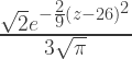
>>> Density(T)

You’ll see that as x gets away from the mean, 30, the probability starts to drop off rapidly. The speed of the drop off is moderated by 2 times the square of the standard deviation, 18, present in the denominator of the exponent.

We’ll call this curve the prior distribution of T. Prior to what you might ask? Prior to me going outside with a thermometer to measure the actual temperature.

---

My thermometer is small and the lines are very close together. This makes it difficult to get a precise measurement. I think I can only measure the temperature to the nearest one or two degrees. We’ll describe this measurement noise by another Normal Random Variable with standard deviation 1.5.

>>> noise = Normal(0, 1.5)
>>> Density(noise)

Before I go outside lets think about the value I might measure on this thermometer. Given our understanding of the temperature we expect to get a value around 30C. This value might vary though both because our original estimate of T might be off (the weather might actually be 33C) and because I won’t measure it correctly because the lines are small. We can describe this value+variability as the sum of two random variables

>>> observation = T + noise

---

Ok, I just came back from outside. I measured 26C on the thermometer; reasonable but a bit lower than I expected. We remember that this measurement has some uncertainty attached to it due to the noise and represent it with a random variable rather than just a number

>>> data = 26 + noise

Note how the data curve looks skinnier. This is because its more precise around the mean value, 26. It’s taller so that the area under the curve is equal to one.

---

After we make this measurement how should our estimate of the temperature change? We have the original estimate, 30C +- 3C, and the new measurement 26C +- 1.5C. We could take the thermometer’s reading because it is more precise but this doesn’t use the original information at all. The old measurement still has useful information and it would be best to cleanly assimilate the new bit of data (26C+-1.5C) into our prior understanding (30C +-3C).

This is the problem of Data Assimilation. We want to assimilate a new meaurement (data) into our previous understanding (prior) to form a new and better-informed understanding (posterior). Really, we want to compute

<<T_new =  T_old given that observation == 26  >>

We can do this in SymPy as follows

>>> T_new = Given( T , Eq(observation, 26) )

This posterior is represented below both visually and mathematically

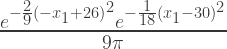
The equation tells us that the temperature, here represented by , drops off both as it gets away from the prior mean 30C and as it gets away from the measured value 26C. The value with maximum likelihood is somewhere between. Visually it looks like the blue curve is described by  27C +- 1.3C or so.

---

We notice that the posterior is a judicious compromise between the two, weighting the data more heavily because it was more precise. The astute statistician might notice that the variance of the posterior is lower than either of the other two (the blue curve is skinnier and so varies less). That is, by combining both measurements we were able to reduce uncertainty below the best of either of them. It’s worth noting that this solution wasn’t built into SymPy-stats or into some standard probabilistic trick. This is the answer given the most basic and fundamental rules.

---

The code for this demo is available here. It depends this statistics branch of SymPy and on matplotlib for the plotting .

---

Data assimilation is a very active research topic these days. Common applications include weather prediciton, automated aircraft navigation, and phone-gps navigation.

Phone/GPS navigation is a great example. Your phone has three ways of telling where it is; cell towers, GPS satellites, and the accelerometer. Cell towers are reliable but low precision.  GPS satellites are precise to a few meters but need some help to find out generally where they are and update relatively infrequently. The accelerometer has fantastic, real-time precision but is incapable of large scale location detection. Merging all three types of information on-the-fly creates a fantastic product that magically tells us to “turn left here” at just the right time.